📊 Statistical Simulation & Naïve Bayes Classifier

Overview

This project was completed for my electrical engineering probability and statistics coursework. The assignment combined theory, simulation, and data analysis to explore how probability models behave in practice.

I used Python to simulate fair and unfair dice, compare simulated results against theoretical probabilities, estimate unknown Gaussian parameters using maximum likelihood estimation, build a Naïve Bayes classifier, and visualize the Central Limit Theorem through repeated sampling.

Project Components

• Simulated fair and unfair 10-sided dice using Monte Carlo methods.
• Compared empirical probabilities against theoretical probability results.
• Estimated Gaussian mean and standard deviation using maximum likelihood estimation.
• Plotted histograms and overlaid fitted Gaussian probability density functions.
• Estimated probability mass functions from demographic purchase data.
• Built a Naïve Bayes classifier to predict whether a user would buy a product.
• Used simulations to visualize how sample means converge under the Central Limit Theorem.

Monte Carlo Simulation

The first part of the project used repeated random trials to estimate the probability of rolling an odd number on a 10-sided die. As the number of trials increased, the simulated probability approached the theoretical result.

import random

t_values = [50, 100, 1000, 2000, 3000, 10000, 100000]

for t in t_values:
    odd_count = 0

    for i in range(t):
        roll = random.randint(1, 10)

        if roll % 2 == 1:
            odd_count += 1

    odd_probability = odd_count / t
    print(f"{t} tosses: P(odd) ≈ {odd_probability}")

Maximum Likelihood Estimation

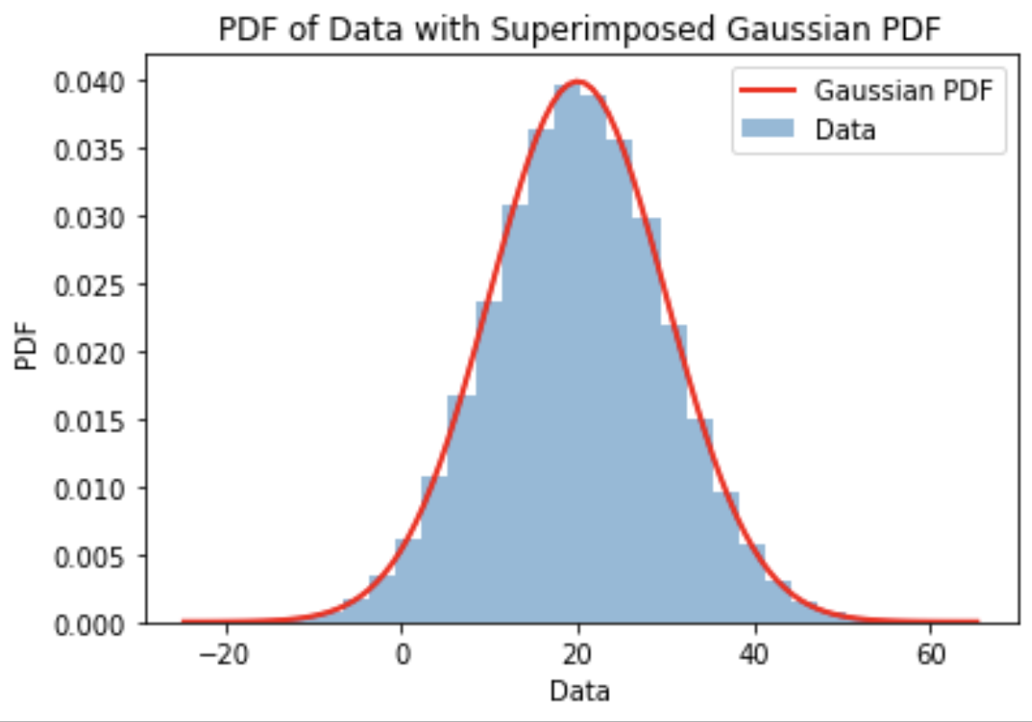
Another section estimated the unknown mean and standard deviation of a normally distributed dataset. Using maximum likelihood estimation, the best-fit Gaussian parameters were computed from the observed data.

import numpy as np

data = np.loadtxt("data.txt")

mu_mle = np.mean(data)
sigma_mle = np.sqrt(np.mean((data - mu_mle) ** 2))

print("mu_MLE:", mu_mle)
print("sigma_MLE:", sigma_mle)

Placeholder for MLE histogram and fitted Gaussian plot:

Naïve Bayes Classifier

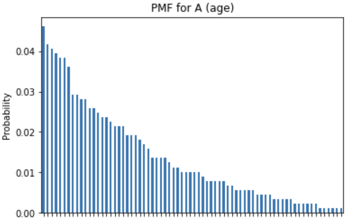
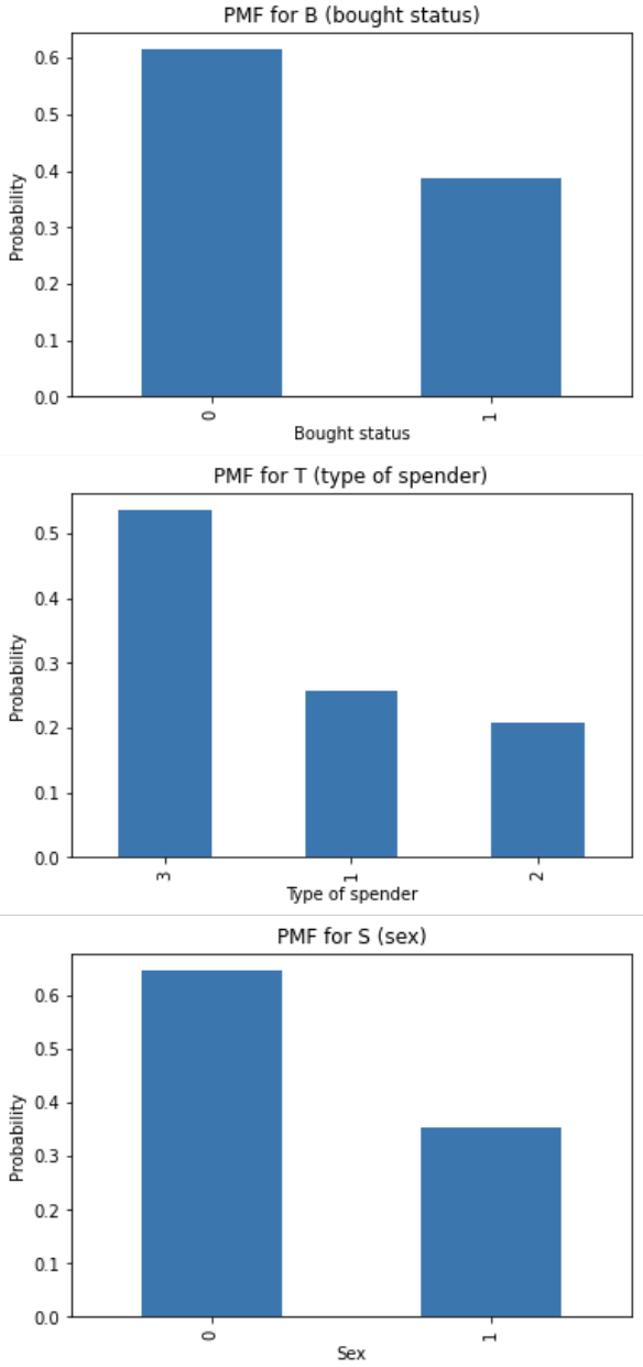
The project also included a Naïve Bayes classifier using demographic purchasing data. The classifier estimated probability mass functions and conditional probability mass functions for features like spender type, sex, and age, then used those probabilities to predict whether a user would buy a product.

import pandas as pd

df = pd.read_csv("user_data.csv")

P_B_1 = sum(df["Bought"]) / len(df)
P_B_0 = 1 - P_B_1

P_T_1 = sum(df["Spender Type"] == 1) / len(df)
P_S_0 = sum(df["Sex"] == 0) / len(df)
P_A_lt_55 = sum(df["Age"] < 55) / len(df)

print("P(B=1):", P_B_1)
print("P(B=0):", P_B_0)

Placeholder for PMF and conditional PMF plots:

Central Limit Theorem Simulation

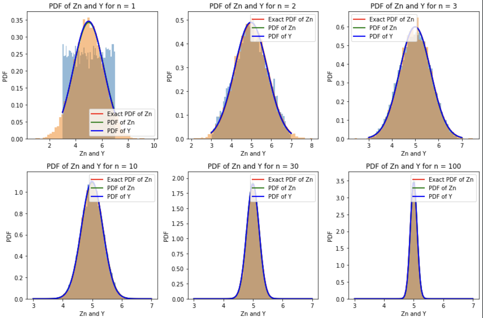
The final part simulated repeated sample means from a uniform distribution and from an unfair die distribution. The plots showed how the distribution of sample means becomes increasingly Gaussian-shaped as the sample size grows.

import numpy as np
import matplotlib.pyplot as plt
from scipy.stats import uniform

a = 3
b = 7
n_values = [1, 2, 3, 10, 30, 100]
t = 10_000

for n in n_values:
    X = uniform.rvs(loc=a, scale=b-a, size=(n, t))
    Zn = np.mean(X, axis=0)

    plt.hist(Zn, density=True, bins=50)
    plt.title(f"PDF of Zn for n = {n}")
    plt.xlabel("Zn")
    plt.ylabel("PDF")
    plt.show()

Placeholder for Central Limit Theorem plots:

What I Learned

• How simulation can validate theoretical probability results.
• How increasing sample size improves the accuracy of empirical estimates.
• How maximum likelihood estimation fits model parameters to observed data.
• How probability mass functions and conditional probabilities support classification.
• How the Central Limit Theorem appears visually through repeated sampling.
• How Python tools like NumPy, Pandas, Matplotlib, and SciPy support statistical analysis.

Reflection

While this was a coursework project, it helped connect probability theory with practical computation. It gave me experience turning mathematical formulas into simulations, visualizations, and classifiers, which is useful for data analysis, signal processing, machine learning, and engineering decision-making.